Interactive Widgets
Jupyter widgets enable interactive data visualization in the Jupyter notebooks.
Notebook Widgets
Notebooks come alive when interactive widgets are used. Users can visualize and control changes in the data. Learning becomes an immersive, plus fun, experience. Researchers can easily see how changing inputs to a model impacts the results.
A library for creating simple interactive maps with panning and zooming, ipyleaflet supports annotations such as polygons, markers, and more generally any geojson-encoded geographical data structure.
Example
from ipyleaflet import Map
Map(center=[34.6252978589571, -77.34580993652344], zoom=10)Installation
With conda:conda install -c conda-forge ipyleafletpip install ipyleafletjupyter nbextension enable --py --sys-prefix ipyleafletjupyter labextension install @jupyter-widgets/jupyterlab-manager jupyter-leafletA Jupyter widget to interactively view molecular structures and trajectories.
Example
import pytraj as pt
import nglview as nv
traj = pt.load('sim.nc', top='sim.prmtop')
traj.strip(":TIP3")
view = nv.show_pytraj(traj)
view.clear()
view.add_cartoon('protein', color_scheme='residueindex')
view.add_ball_and_stick('not protein', opacity=0.5)
viewInstallation
With conda:conda install -c bioconda nglviewpip install nglview
jupyter nbextension enable --py --sys-prefix nglviewK3D lets you create 3D plots backed by WebGL with high-level API (surfaces, isosurfaces, voxels, mesh, cloud points, vtk objects, volume renderer, colormaps, etc). The primary aim of K3D-jupyter is to be easy for use as stand alone package like matplotlib, but also to allow interoperation with existing libraries as VTK. The power of ipywidgets makes it also a fast and performant visualisation tool for HPC computing e.g. fluid dynamics.
Showcase gallery: https://k3d-jupyter.org/gallery/index.html.
Example
import k3d
import numpy as np
lines = np.load('vertices.npy')
lines_attributes = np.load('attributes.npy')
plot = k3d.plot()
for l, a in zip(lines, lines_attributes):
plot += k3d.line(l, attribute=a, width=0.0001,
color_map=k3d.matplotlib_color_maps.Inferno, color_range=[0,0.5], shader='mesh',
compression_level=9)
plot.display()Installation
With pip:pip install k3d
jupyter nbextension enable --py --sys-prefix k3djupyter labextension install @jupyter-widgets/jupyterlab-manager k3dA 2-D interactive data visualization library implementing the constructs of the grammar of graphics, bqplot provides a simple API for creating custom user interactions.
Example
import numpy as np
import bqplot.pyplot as plt
size = 100
plt.figure(title='Scatter plot with colors')
plt.scatter(np.random.randn(size), np.random.randn(size), color=np.random.randn(size))
plt.show()Installation
With conda:conda install -c conda-forge bqplotpip install bqplotjupyter nbextension enable --py --sys-prefix bqplotjupyter labextension install @jupyter-widgets/jupyterlab-manager bqplotA 3-D visualization library enabling GPU-accelerated computer graphics in Jupyter.
Example
from pythreejs import *
f = """
function f(origu,origv) {
// scale u and v to the ranges I want: [0, 2*pi]
var u = 2*Math.PI*origu;
var v = 2*Math.PI*origv;
var x = Math.sin(u);
var y = Math.cos(v);
var z = Math.cos(u+v);
return new THREE.Vector3(x,y,z);
}
"""
surf_g = ParametricGeometry(func=f, slices=16, stacks=16)
surf = Mesh(geometry=surf_g, material=MeshLambertMaterial(color='green', side='FrontSide'))
surf2 = Mesh(geometry=surf_g, material=MeshLambertMaterial(color='yellow', side='BackSide'))
c = PerspectiveCamera(position=[5, 5, 3], up=[0, 0, 1],
children=[DirectionalLight(color='white',
position=[3, 5, 1],
intensity=0.6)])
scene = Scene(children=[surf, surf2, c, AmbientLight(intensity=0.5)])
Renderer(camera=c, scene=scene, controls=[OrbitControls(controlling=c)], width=400, height=400)Installation
With conda:conda install -c conda-forge pythreejspip install pythreejsjupyter nbextension enable --py --sys-prefix pythreejsjupyter labextension install @jupyter-widgets/jupyterlab-manager jupyter-threejs3-D plotting for Python in the Jupyter notebook based on IPython widgets using WebGL.
Example
import ipyvolume.pylab as p3
import numpy as np
fig = p3.figure()
q = p3.quiver(*stream.data[:,0:50,:200], color="red", size=7)
p3.style.use("dark") # looks better
p3.animation_control(q, interval=200)
p3.show()Installation
With conda:conda install -c conda-forge ipyvolumepip install ipyvolume
jupyter nbextension enable --py --sys-prefix ipyvolumejupyter labextension install @jupyter-widgets/jupyterlab-manager jupyter-threejs ipyvolumeBeakerX includes widgets for interactive tables, plots, forms, Apache Spark, and more. The table widget automatically recognizes pandas dataframes and allows you to search, sort, drag, filter, format, select, graph, hide, pin, and export to CSV or clipboard. This makes connecting to spreadsheets quick and easy.
The table widget, shown below, is so fast because it's implemented with the PhosphorJS Data Grid, part of Jupyter Lab's architecture.
Example
import pandas as pd
from beakerx import *
pd.read_csv("UScity.csv")Installation
With conda:conda install -c conda-forge beakerx ipywidgetspip install beakerx
beakerx-installGmaps lets you embed interactive Google maps in Jupyter notebooks. Visualize your data with heatmaps, GeoJSON, symbols and markers, or plot directions, traffic, or cycle routes. Let users draw on the map and capture the coordinates of the markers or polygons they are placing to build interactive applications entirely in Python.
Example
import gmaps
import gmaps.datasets
gmaps.configure(api_key="AI...") # Your Google API key
locations = gmaps.datasets.load_dataset("taxi_rides")
fig = gmaps.figure()
# locations could be an array, a dataframe or just a Python iterable
fig.add_layer(gmaps.heatmap_layer(locations))
figInstallation
With conda:conda install -c conda-forge gmapspip install gmaps
jupyter nbextension enable --py --sys-prefix gmapsjupyter labextension install @jupyter-widgets/jupyterlab-managerThe Jupyter widget framework is extensible and enables developers to create custom widget libraries and bindings for visualization libraries of the JavaScript and TypeScript ecosystem.
The cookiecutter projects help widget authors get up to speed with the
packaging and distribution of Jupyter interactive widgets, in
JavaScript and
TypeScript.
They produce a base project for a Jupyter interactive widget library following the current best practices. An implementation for a placeholder "Hello World" widget is provided. Following these practices will help make your custom widgets work in static web pages (like the examples of this page) and be compatible with future versions of Jupyter.
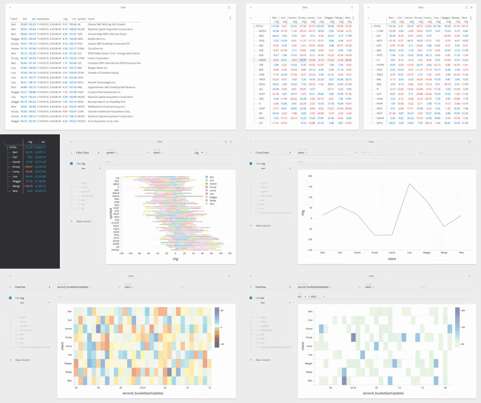
Perspective is an interactive visualization component for large, real-time datasets. Originally developed for J.P. Morgan's trading business, Perspective makes it simple to build real-time & user configurable analytics entirely in the browser, or in concert with Python and/or Jupyterlab.
Perspective can be used to create reports, dashboards, notebooks and applications, with static data or streaming updates via Apache Arrow..
